Matrix Factorization

Matrix factorization은 simple embedding model이다. feedback matrix(m x n)가 주어졌을때, m은 users의 수, n은 items의 수:

• user embedding matrix를 U (m x d), row i는 user i의 embedding
• item embedding matrix를 V (n x d), row j는 item i의 embedding

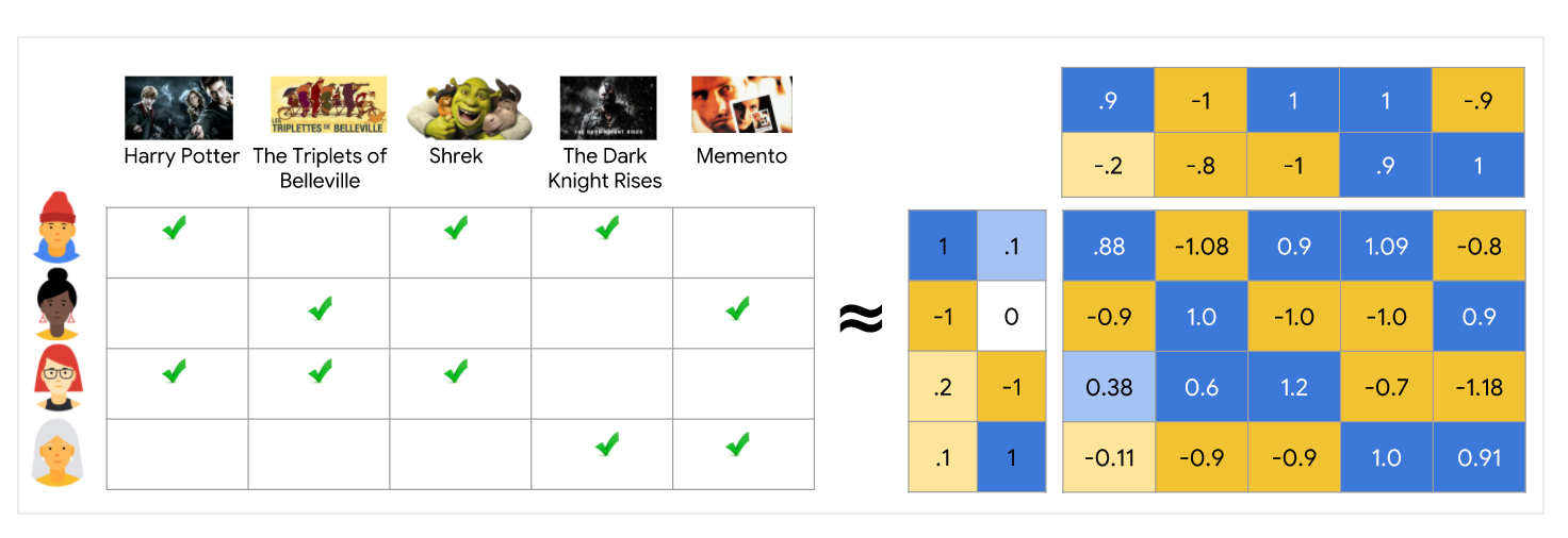
임베딩은 UV^T가 feedback matrix A의 좋은 근사치가 되도록 학습이 된다. U dot V ^T의 (i, j) entry는A_i,j 에 가까워지기를 원하는 user i, item j의 embedding의 <U_i V_j>의 dot product 이다.

Matrix factorization은 일반적으로 full matrix를 학습하는 것보다 더 간결한 표현(compact representation)을 제공한다. full matrix O(nm) 항목이 있고, 임베딩 matrices U, V에는 O((n+m)d) entries가 있습니다. 여기서 임베딩 차원 d는 일반적으로 m, n보다 훨씬 작다. (user, item 별로 m x d, n x d의 행렬이 존재). 결과적으로 matrix factorization은 관측치가 low-dimensional subspace에 가깝다고 가정하여 데이터에서 latent structure를 찾는다. 앞의 예에서 n, m, d의 값이 너무 작아서 이점이 무시될수 있다. 그러나 실제 추천 시스템에서 matrix factorization은 full matrix를 학습하는 것보다 훨씬 더 간결 할 수 있다.

Choosing the Objective Function

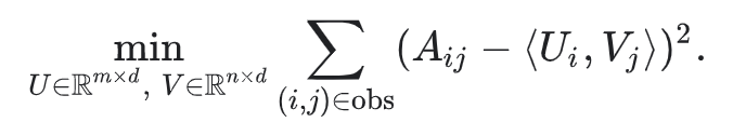
직권적인 objective function 중 하나는 squared distance이다. 관찰된 모든 항목 쌍에 대한 squared errors의 합을 최소화 하면 된다.

이 목적함수에서는 관찰된 (i,j)의 쌍에 대해서만 합산을 한다. 즉 feedback matrix에서의 non-zero values에 대해서만 합. 그러나 하나의 값만 합산하는 것은 좋은 생각이 아니다. 모든 값의 행렬은 손실을 최소화하고 효과적인 추천을 만들 수 없고 제대로 일반회되지 않은 모델을 생성한다.

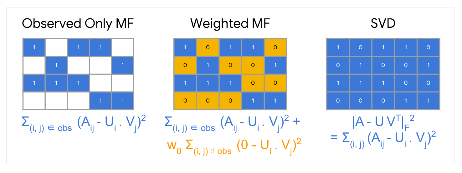
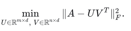
관찰되지 않은 값을 0으로 처리하고 행렬의 모든 entries를 합할 수 있다. 이 방법은 A와 근사 UV^T사이의 squared Frobenius 거리를 최소화하는 것에 해당한다.

행렬의 SVD(Singular Value Decomposition)를 통해 quadratic(2차) 문제를 풀 수 있다. 그러나 실제 애플리케이션에서는 행렬 A가 매우 sparse할 수 있기 때문에 SVD도 좋은 솔루션이 아니다. 예를 들어 특정 사용자가 본 모든 동영상과 비교하여 Youtube의 모든 동영상을 생각해보자. 솔루션 UV^T (입력 매트릭스의 모델 근사값에 해당하는)는 0에 가까워 일반화 성능이 저하 될 수 있다.

반대로 Weighted Matrix Factorization은 objective를 다음 두 합계로 분해 한다.

• 관찰된 항목의 합계
• 관찰되지 않은 항목에 대한 합계 (0으로 처리)

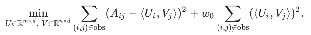
여기서 w₀은 objective가 둘 중 하나에 의해 지배(dominant)되지 않도록 두 항에 가중치를 부여하는 hyperparameter 이다. 이 파라미터를 조정하는 것은 매우 중요.

실제 applications에서 관찰 된 쌍에 신중하게 가중치를 부여핸야 한다. 예를 들어서 frequent items(ex: extremely popular YouTube videos) 또는 frequent queires(ex: heavy users) 는 아마도 objective function을 지배 할 수 있다. item frequency를 설명하기 위해 훈련 예제에 가중치를 부여하여 이 효과를 수정 할 수 있다. 즉, 목적함수를 다음으로 대체 할 수 있다.

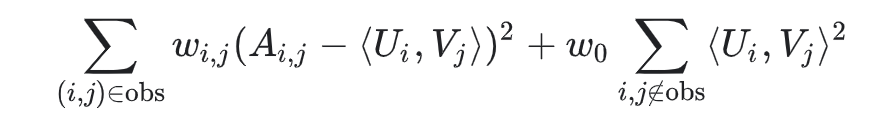
w_i,j은 query i, item j의 frequency의 함수

Minimizing the Objective Function

목적 함수를 최소화하는 일반적인 알고리즘은 다음과 같다.

• Stochastic gradient descent (SGD) 는 손실 함수를 최소화하는 일반적인 방법
• Weighted Alternating Least Squares (WALS)는 특정 목표에 특화되어 있는 방법

목적은 두 행렬 U, V 각각에서 quadratic 이다. (그러나 문제가 jointly convex는 아니다.) WALS는 임베딩을 무작위로 초기화 한 다음 아래 과정을 번갈아 가면서 한다.

• U를 고정하고 V를 계산
• V를 고정하고 U를 계산

각 단계(stage)는 linear system의 솔루션을 통해 정확하게 해결할 수 있으며 배포가 가능하다. 이 기술은 각 단계가 손실을 줄이기 위해 보장되기 때문에 수렴이 보장된다.

SGD vs WALS

• SGD와 WALS는 장단이 있다. 아래 정보를 검토하여 비교 방법을 확인
• SGD
  • (장점) Very Flexible - can use other loss functions
  • (장점) Can be parallelized
  • (단점) Slower = does not converge as quickly
  • (단점) Harder to handle the unobserved entries ( need to use negative sampling or gravity)
• WALS
  • (단점) Loss Squares에만 의존
  • (장점) Can be parallelized
  • (장점) Converges faster than SGD.
  • (장점) Easier to handle unobserved entries

참고

• https://developers.google.com/machine-learning/recommendation/collaborative/matrix